Excel is an indispensable tool for professionals across a wide range of industries when it comes to data analysis and reporting. Excel provides users with a wide range of features and functionality that allow them to manipulate and analyze data easily and precisely.
GETPIVOTDATA is one such function that is specifically designed for extracting data from pivot tables.
In this article, we’ll explore the intricacies of the GETPIVOTDATA function and provide a comprehensive guide on how to leverage its capabilities effectively.


Understanding GETPIVOTDATA:
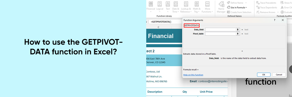
GETPIVOTDATA is a built-in Excel function that allows users to retrieve data from a pivot table based on specific criteria. It eliminates the need for manually referencing cells within a pivot table, providing a more structured and dynamic approach to data retrieval. The syntax of the GETPIVOTDATA function is as follows:
| GETPIVOTDATA(data_field, pivot_table, [field1, item1, field2, item2, …]) |
- data_field: The name of the field (column) in the pivot table from which to retrieve data.
- pivot_table: A reference to any cell in the pivot table.
- [field1, item1, field2, item2, …]: Optional. Pairs of field names and items that define the criteria for data retrieval.
Practical Applications:
1. Basic Data Retrieval:
The simplest application of GETPIVOTDATA involves retrieving data based on a single criterion. For example, to extract the total sales amount from a pivot table where “Sales” is the data field, you can use the following formula:
| =GETPIVOTDATA(“Sales”, A1) |
Here, A1 is a reference to any cell within the pivot table. Excel will return the total sales amount from the pivot table.
2. Retrieval with Multiple Criteria:
GETPIVOTDATA also allows users to specify multiple criteria for data retrieval. This is particularly useful when dealing with complex datasets. For instance, to retrieve the sales amount for a specific product (“Product A”) and region (“North”), you can use the following formula:
| =GETPIVOTDATA(“Sales”, A1, “Product”, “Product A”, “Region”, “North”) |
This formula instructs Excel to retrieve the sales amount for “Product A” in the “North” region from the pivot table.
3. Dynamic Data Extraction:
One of the key advantages of GETPIVOTDATA is its ability to dynamically retrieve data based on changing criteria. By referencing cells containing criteria values, you can create dynamic reports that update automatically as the criteria change. For example, you can link dropdown lists or input cells to the criteria fields in your GETPIVOTDATA formulas, allowing users to interactively explore the data.
4. Error Handling:
GETPIVOTDATA also provides error handling capabilities to deal with situations where the specified criteria do not match any data in the pivot table. You can use the IFERROR function to handle such errors gracefully and display custom messages or alternative values.
Tips for Effective Use:
1. Understand the Pivot Table Structure:
Before using GETPIVOTDATA, it’s essential to familiarize yourself with the structure of the pivot table, including the field names and items. This will help you construct accurate GETPIVOTDATA formulas and retrieve the desired data efficiently.
2. Use Descriptive Field Names:
When specifying criteria in GETPIVOTDATA formulas, use descriptive field names and item labels to ensure clarity and accuracy. This will make your formulas easier to understand and maintain, especially in complex pivot table setups.
3. Experiment with Criteria Combinations:
Don’t hesitate to experiment with different combinations of criteria in your GETPIVOTDATA formulas to extract specific subsets of data from the pivot table. This flexibility allows you to tailor your reports to meet various analytical requirements.
4. Test and Validate Formulas:
Before finalizing your reports, thoroughly test and validate your GETPIVOTDATA formulas to ensure they are retrieving the correct data. Check for accuracy by comparing the results with manual calculations or sample data from the pivot table.
Also check out our articles on Excel dashboard
Conclusion:
The GETPIVOTDATA function in Excel is a powerful tool that streamlines the process of data retrieval from pivot tables. Its capabilities enable users to extract precise and dynamic data based on specific criteria, thus facilitating informed decision-making and analysis. Whether you’re creating interactive dashboards, dynamic reports, or ad-hoc analyses.
GETPIVOTDATA lets you discover the insights hidden in your pivot tables in an efficient and easy way. By understanding Excel’s syntax and practical applications, you can improve your data analysis skills and make use of its powerful features.


